Data Analysis Using R

This file contains basic instructions for data anlysis using R.

R is a programming language and free software environment for statistical computing and graphics. It is supported by the R Core Team and the R Foundation for Statistical Computing. It is widely used among statisticians and data miners for developing statistical software and data analysis.

Table of contents

• Data Analysis Using R
  • Table of contents
  • Basics of R
  • Common Commands for Data Management
  • Data Visualitation and Graphics
    • Using built in R functions
    • Using ggplot2
  • Stastistical Tools

Basics of R

• Installing R Studio

  R -Studio can be downloaded using the link: Download R-Studio

• Related Book : R for Data Science

• Importing Data

  read.table("data or link")
  #Here is the example of importing data that is saved in same directory as R.script
  
  my_data = read.csv("my_data.csv")
    
  # this will import and save my_data.csv from the computer as my_data
    
  
  #here is the example of importing data online 
  my_data1 = read.table("url")
  my_data1 = read.table("http://www.stat.wmich.edu/naranjo/EMdatasets/btt.txt")
  
  #This will import data from "http://www.stat.wmich.edu/naranjo/EMdatasets/btt.txt" and save as my_data1
  

  Note: If you are importing file from computer, make sure the file to be imported is on same directory as R.script. OTHERWISE it will show error.

• Exporting Data

    #.txtfile
    write.table(my_data1, file = "my_data1_exported.txt") # export my_data1 in .txt file in same directorey as R. file.
  
    #.csv file
    write.table(my_data1, file = "my_data1_exported.csv") # exports my_data1 in csv format
    write.table(my_data1, file = "my_data1_exported.csv", sep = ",") #exports my_data1 in csv format with separation using comma.
  

• Creating matrix and naming variables

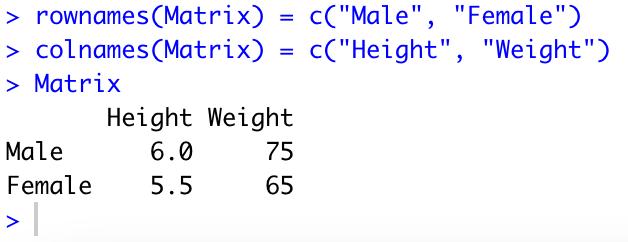
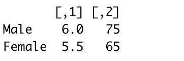
  # Assume two variables average Height (foot) and average weight (kg) for male and female as below:
  Matrix = matrix(c(6, 75, 5.5, 65), nrow =2 , ncol = 2, byrow = T) # creates a matrix with 2 rows and 2 columns.
  

  

  rownames(Matrix) = c("Male", "Female") # adds names to row
  colnames(Matrix) = c("Height", "Weight") #adds names to columns
  Matrix
  

  

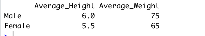
  Male = c(6, 75)
  Female = c(5.5, 65)
  matrix1 = (rbind(Male, Female)) #combines male and female observation creating a matrix
  matrix1
  

  

  colnames(matrix1) = c("Average_Height", "Average_Weight")
  matrix1
  

  

• Naming columns/variables for imported file

  #Assume a dataset called data has variables V1, V2, and V3, the columns can be named as follows:
  names(data) = c("V1", "V2", "V3")
    
  my_data1 = read.table("http://www.stat.wmich.edu/naranjo/EMdatasets/btt.txt")
  
  #for our dataset, variables are: "childid", "sex", "bweight", "gestage", "momage", "parity", "mdbp", "msbp", "momeduc", "mmedaid", "socio", "dbp5", "sbp5", "ht5", "wt5", "hdl5", "ldl5", "trig5", "smoke5", "medaid5", "socio5"
  
  names(my_data1) = c("childid", "sex", "bweight", "gestage", "momage", "parity", "mdbp", "msbp", "momeduc", "mmedaid", "socio", "dbp5", "sbp5", "ht5", "wt5", "hdl5", "ldl5", "trig5", "smoke5", "medaid5", "socio5")
  
  #function head will give only first few observation for all variables.
  
  head(my_data1)
  #output
  

  

Common Commands for Data Management

• Finding number of observations: nrow(data) and number of variable: ncol(data) in a certain dataset: data

  nrow(data) # gives total number of rows in the dataset-data. It is also the total number of observationsin the data set data.
  
  ncol(data) # gives total number of columns in the data set-data. It is also the total number of variables in the data set data. 
  
  dim(data) # gives the total number of rows and columns at once
  

  The number of observation in the data set is number of rows and number of variables is number of columns.

• Acessing particular variable (column) or/and observation (row)

  #let assume we have a dataset: data and it has column V1, V2, and V3 as three variables. 
  data$V1 # acesses the data in vairable V1 from dataset: data
  
  data[,c("V1")] # acesses V1 only
  data[,c("V1", "V2")] #acesses V1 and V2 from data
    
  #Using my_data1
  my_data1[, c("childid")] # will acess childid only from my_data1
  
  my_data1[, c("childid", "socio5", "momeduc")] #will acess childid, socio5, and mumeduc variable form my_data1
  
  my_data1[1:10,] #will acess first 10 rows and all variables
  
  my_data1[1:10, 1:5] #will acess first 10 rows/observations and first 5 variables or column
  
  my_data1[20:40, c(1,3,5,6)] #will acess observation from 20-40 and varibles at position 1, 3, 5, and 6.
  
  #mydata[rows, columns] general format
  
  #selecting specific value/variables:
  my_data1[my_data1$sex == 2,] # gives data that has childid greater than 50
  
  my_data1[my_data1$sex == 2 & my_data1$childid >=50,] # gives data for which sex is equal to 2 and childid is greater than or equal to 50
  

• Data management using Tidyverse

  install.packages("tidyverse") #will install tidyverse package that has multiple packages for data management
  

1. Adding a different variable or column to a dataset: mutate(data,new_var = )

    library(tidyverse) #packages shouls be loaded before use
       
    my_data2 = mutate(my_data1, ratio = childid/momeduc) # This creates a new data set with a variable called ratio that equal the ratio of childid/momeduc while preserving all other variable form dataset: my_data1
   
    my_data1 = mutate(my_data1, ratio1 = childid * momeduc *5) #This adds a new variable called ratio 1 in the same data set.
   

   Make sure you load the specific package before you use specific commands form it.

2. Selecting specific variables and creating new data set select()

   library(tidyverse)
   
   select(my_data1, c("childid", "socio5", "mumeduc")) #This select only childid, socio5, and mumeduc.
   
   my_data2 = select(my_data1, c("childid", "socio5", "mumeduc")) #This creates a new dataset: my_data2 with only three variable
   

3. Selecting specific data based on given condition `filter(data, var_condition)’

   filter(my_data1, sex ==2) # gives data for all variables in data set: my_data1 for which sex is 
   
   filter(my_data1, childid>=50) # gives data for all variables in data set: my_data1 for which childid is equal or greater than 50
   

4. Use of pipe (%>%) to filter and many more

   my_data1 %>%
   filter(childid >=50)) # will do as in previous code
   
   my_data1%>%
   filter(childid >= 50) %>%
   select(c("childid", "socio5", "momeduc")) # will first filter the data for which childid is greater than or equal to 50 and selects three variables: childid, socio5, and momeduc from my_data1. Using pipe we can operate multiple function in single operation.
   

Data Visualitation and Graphics

Using built in R functions

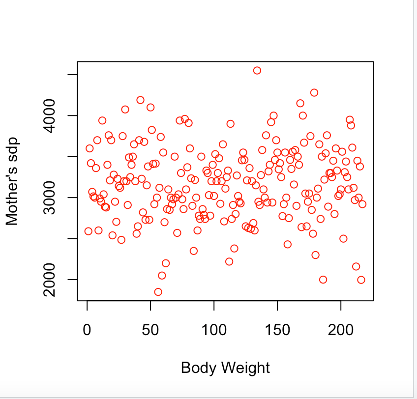
1. Scatter plot plot(x,y)

   plot(my_data1$bweight,my_data$msdp)
   

   

• Adding labels and colors

   #Adding labels
  plot(my_data1$bweight,my_data1$msdp, xlab = "Body Weight", ylab = "Mother's sdp", col = "red")
  

  

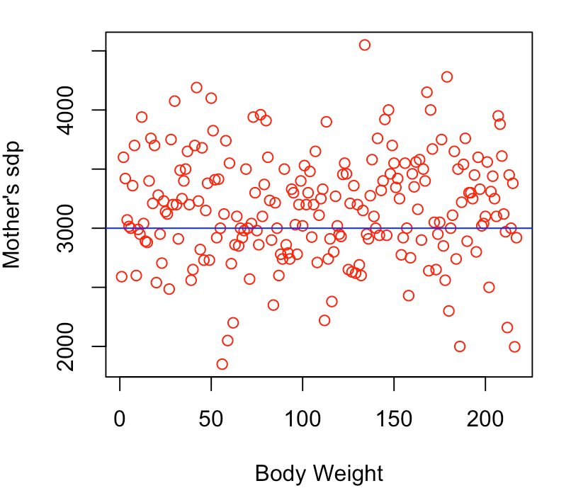
  #Adding abline
    
  plot(my_data1$bweight,my_data1$msdp, xlab = "Body Weight", ylab = "Mother's sdp", col = "red")
    abline(h = 3000, col = "blue") # will add a reference line at mothers sds = 3000
  

  

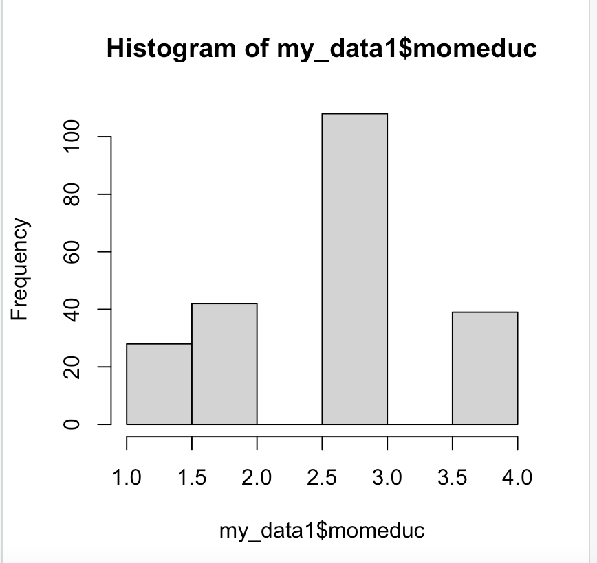
1. Histogram hist(data$var)

   hist(my_data1$momeduc)
   

   

• Adding labels and colors

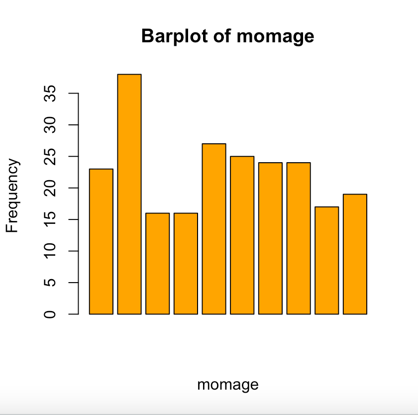
1. Bar plot barplot(data$var, xlab = " ", ylab = " ", col = " ")

   barplot(my_data1$momage[1:10],xlab = "momage", ylab = "Frequency", main = "Barplot of momage", col = "orange") # gives barplot for first 10 observation of momage from my_data1. main gives title. This is a big data set and barplot for every observation looks messy. That is why I chose first 10 observations
   

   

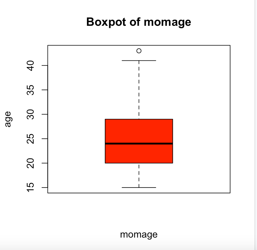
1. Boxplot ` boxplot(data$var, xlab = “”, ylab = “”, main = “”, col = “”)`

   boxplot(my_data1$momage, xlab = "momage", ylab = "Age", main = "Boxpot of momage", col = "red") #plots the boxplot of momage form my_data1
   

   

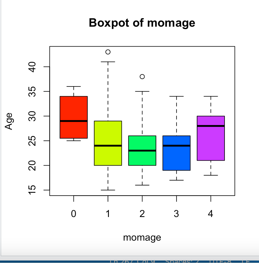
   boxplot(my_data1$momage ~ my_data1$socio5, xlab = "momage", ylab = "Age", main = "Boxpot of momage", col = rainbow(5))  #plots the boxplot of momage by socio5 form my_data1. col = rainbow(n) gives different color and n is number of color determined by number of boxplot
   

   

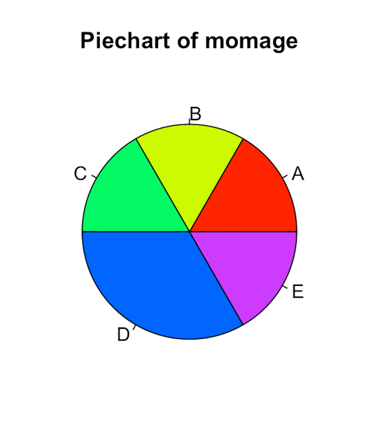
2. Piechart `pie(data$var, xlab = “”, radious = “”, main = “”, col = “”, clockwise)

   pie(my_data1$socio5[1:5], labels = c("A", "B", "C", "D", "E"), main = "Piechart of momage", col = rainbow(5)) # creates piechart for first five observation of socio 5.
   

   

Using ggplot2

Stastistical Tools